Generate metadata from column names
In the example dataset proteinGroups_Cbl, protein intensities are found in data columns whose names start with “Intensity”. We identify such columns using grep()
idx_intensity_columns <- grep("^Intensity.", names(proteinGroups_Cbl))
print(names(proteinGroups_Cbl)[idx_intensity_columns][1:10])
## [1] "Intensity.Cbl_0_Ech1_R1" "Intensity.Cbl_0_Ech1_R2"
## [3] "Intensity.Cbl_0_Ech1_R3" "Intensity.Cbl_0_Ech2_R1"
## [5] "Intensity.Cbl_0_Ech2_R2" "Intensity.Cbl_0_Ech2_R3"
## [7] "Intensity.Cbl_0_Ech3_R1" "Intensity.Cbl_0_Ech3_R2"
## [9] "Intensity.Cbl_0_Ech3_R3" "Intensity.Cbl_030_Ech1_R1"Intensity columns are usually named using a pattern. Here the names of the cell type, of the experimental condition (time of stimulation), of the biological replicate and of the technical replicate are separated by the character _. We can use the function identify_conditions() to map conditions from intensity column names:
condition <- identify_conditions(proteinGroups_Cbl,
                                  Column_intensity_pattern = "^Intensity.",
                                  split = "_",
                                  bckg_pos = 1,
                                  time_pos = 2,
                                  bio_pos = 3,
                                  tech_pos = 4)
summary(condition)
## column bckg time bio tech
## Intensity.Cbl_0_Ech1_R1: 1 Cbl:45 0 :18 Ech1:30 R1:30
## Intensity.Cbl_0_Ech1_R2: 1 WT :45 030:18 Ech2:30 R2:30
## Intensity.Cbl_0_Ech1_R3: 1 120:18 Ech3:30 R3:30
## Intensity.Cbl_0_Ech2_R1: 1 300:18
## Intensity.Cbl_0_Ech2_R2: 1 600:18
## Intensity.Cbl_0_Ech2_R3: 1
## (Other) :84Import custom metadata
You can also import this metadata from a separate file. The package comes with one such file.
condition_custom <- read.csv( system.file("extdata", "proteinGroups_Cbl_metadata.csv", package = "InteRact") )
summary(condition_custom)
## name Cell.type Stim.time Bio.rep
## Intensity.Cbl_0_Ech1_R1: 1 CBL-OST :45 t=030s:18 Sample 1:30
## Intensity.Cbl_0_Ech1_R2: 1 Wild-type:45 t=0s :18 Sample 2:30
## Intensity.Cbl_0_Ech1_R3: 1 t=120s:18 Sample 3:30
## Intensity.Cbl_0_Ech2_R1: 1 t=300s:18
## Intensity.Cbl_0_Ech2_R2: 1 t=600s:18
## Intensity.Cbl_0_Ech2_R3: 1
## (Other) :84
## Tec.rep
## Injection 1:30
## Injection 2:30
## Injection 3:30
##
##
##
## This is the right place to reorder conditions if needed:
Finally, metadata column names must be changed to match those obtained by calling identify_conditions().
As documented for identify_conditions(), column contains intensity column names (as they appear when calling names()), bckg contains the identity of the cell type, time contains the name of the experimental condition, and bio and rep contain the names of the biological and technical replicate respectively.
This custom metadata can then be passed to InteRact():
res <- InteRact(proteinGroups_Cbl,
                bait_gene_name = "Cbl",
                condition = condition_custom,
                bckg_bait = "CBL-OST",
                bckg_ctrl = "Wild-type")
## Contaminant proteins discarded
## Proteins with no gene name available discarded
## Number of theoretically observable peptides unavailable : used MW instead
## Merge protein groups associated to the same gene name (sum of intensities)
## Rescale median intensity across conditions
## Replace missing values and perform interactome analysis for 1 replicates
## Nrep=1
## Averaging 1 interactomesNote that we had to change parameters bckg_bait and bckg_ctrl according to the values taken by condition_custom$bckg. Custom names now appears in the interactome and in subsequent plots (as for instance in the title of volcano plots):
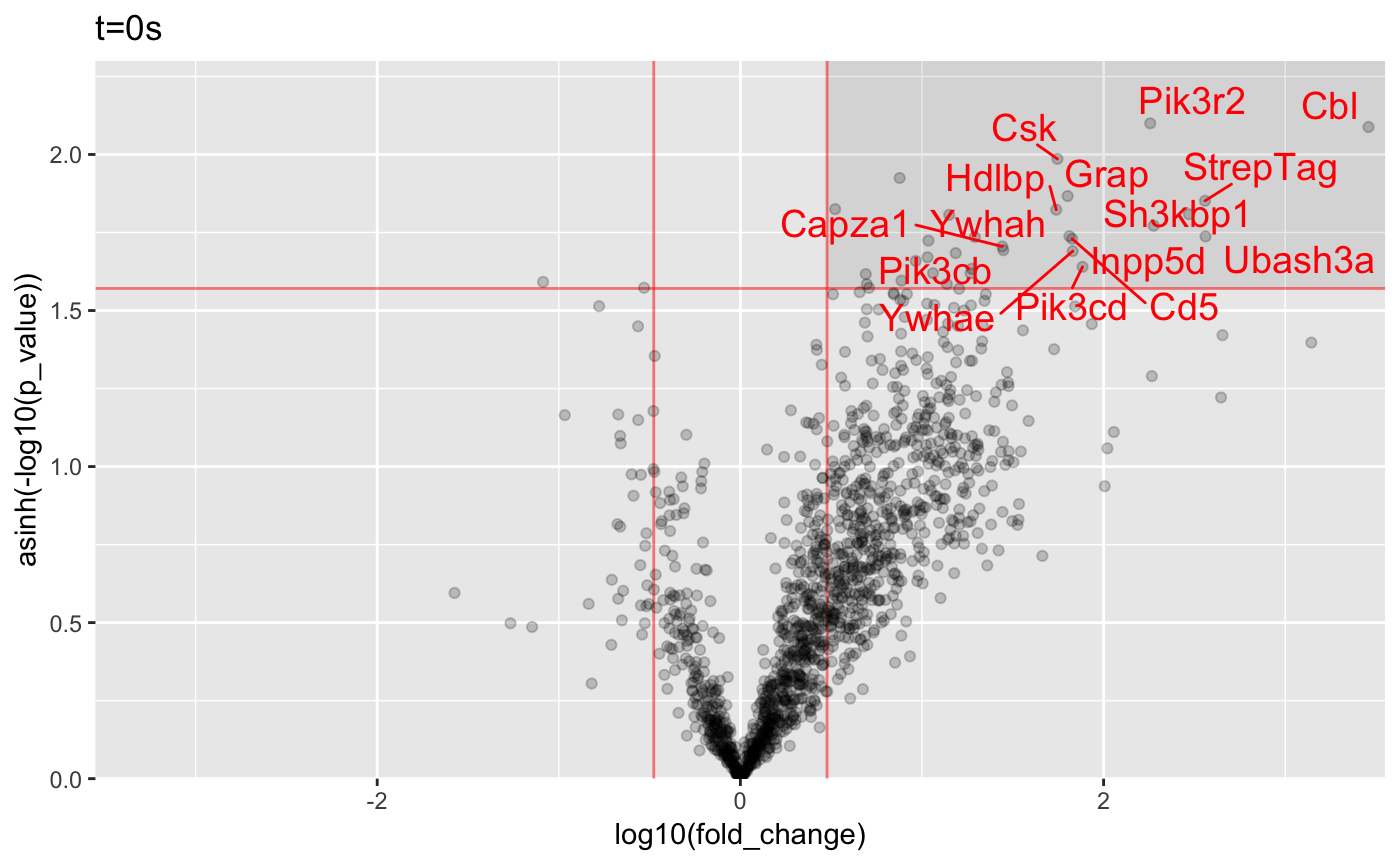
print(res$conditions)## [1] "t=0s" "t=030s" "t=120s" "t=300s" "t=600s"print(res$replicates)## [1] "Sample 1" "Sample 2" "Sample 3"plot_volcanos(res, p_val_thresh = 0.005, fold_change_thresh = 3)[[1]]